Lagrange’s Equations

\[L = T - V\] \[\frac{d}{dt}\left(\frac{\partial L}{\partial \dot{q_i}}\right) - \frac{\partial L}{\partial q_i} = Q_i\]

Where:

• \(T\) is the system’s kinetic energy
• \(V\) is the system’s potential energy
• \(q_i\) represents a coordinate in a system
  • e.g in cartesian \(\mathbb{R}^3\), we have \((q_1, q_2, q_3) = (x, y, z)\)
• \(Q_i\) are the forces acting on the \(i^{th}\) coordinate

Example: Projectile

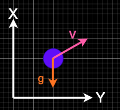
Kinetic Energy, T and Potential Energy, V

\[T = \frac{1}{2}M\dot{x}^2 + \frac{1}{2}M\dot{y}^2\] \[V = Mgy\]

Lagrangian, L

\[L = T - V\] \[L = \frac{1}{2}M\dot{x}^2 + \frac{1}{2}M\dot{y}^2 - Mgy\]

Forces

\[\begin{aligned} drag &= \frac{1}{2}\rho v^2 C_D A \\ &= \frac{1}{2}k_D v^2 \end{aligned}\]

Where:

• \(k_D = \rho C_D A\) is approximately constant

Equations of motion w.r.t x

\[L = \frac{1}{2}M\dot{x}^2 + \frac{1}{2}M\dot{y}^2 - Mgy\] \[\frac{d}{dt}\left(\frac{\partial L}{\partial \dot{x}}\right) - \frac{\partial L}{\partial x} = F_x\] \[\frac{\partial L}{\partial \dot{x}} = M\dot{x}, \frac{d}{dt}\left(\frac{\partial L}{\partial \dot{x}}\right) = M\ddot{x}, \frac{\partial L}{\partial x} = 0\] \[F_x = \frac{1}{2}k_D \dot{x}^2\] \[\therefore M\ddot{x} = \frac{1}{2}k_D \dot{x}^2\]

Equations of motion w.r.t y

\[L = \frac{1}{2}M\dot{x}^2 + \frac{1}{2}M\dot{y}^2 - Mgy\] \[\frac{d}{dt}\left(\frac{\partial L}{\partial \dot{y}}\right) - \frac{\partial L}{\partial y} = F_y\] \[\frac{\partial L}{\partial \dot{y}} = M\dot{y}, \frac{d}{dt}\left(\frac{\partial L}{\partial \dot{y}}\right) = M\ddot{y}, \frac{\partial L}{\partial y} = -Mg\] \[F_y = \frac{1}{2}k_D \dot{y}^2\] \[\therefore M\ddot{y} + Mg = \frac{1}{2}k_D \dot{y}^2\]

State space representation

Rearranging gives:

\[\begin{aligned} \ddot{x} &= -\frac{1}{2M}k_D\dot{x} \\ \ddot{y} &= -g - \frac{1}{2M}k_D\dot{y} \end{aligned}\]

We can now represent this in an ode solver:

import scipy.integrate as integrate
import matplotlib.pyplot as plt
from matplotlib.gridspec import GridSpec
from matplotlib.animation import FuncAnimation
import numpy as np


class Ball():
    def __init__(self, Kd=0.0, M=1.0, g=9.81):
        self.M = M
        self.Kd = Kd
        self.g = g

    def _ode(self, X0, t):
        [x, dx, y, dy] = X0
        drag = self.Kd/(2.0 * self.M)

        return [dx, -drag * dx, dy, -self.g - drag * dy]

    def simulate(self, x_init, t):
        return integrate.odeint(self._ode, x_init, t)


class DrawBall:
    def __init__(self, ax):
        with plt.style.context("dark_background"):
            self.ball, = ax.plot([], [])
            self.path, = ax.plot([], [], linestyle='--', alpha=0.7)
            self.ax = ax
            ax.grid(True, linestyle=":", alpha=0.5)

    def draw(self, x, y):
        phi = np.linspace(-np.pi, np.pi, 32)
        self.ball.set_data(x + np.cos(phi), y + np.sin(phi))
        xd, yd = self.path.get_data()
        if x == 0.0 and y == 0.0:
            xd, yd = [], []
        self.path.set_data(np.append(xd, x), np.append(yd, y))

        self.ax.set_xlim(x - 40, x + 40)
        self.ax.set_ylim(y - 50, y + 50)
        return self.ax,


ball = Ball(Kd=10.0, M=10.0)

T0 = 0.0
TN = 7.0
t = np.linspace(T0, TN, num=5000)

x_init = [0.0, 25.0, 0.0, 50.0]
x = ball.simulate(x_init, t)

with plt.style.context("dark_background"):
    color1 = plt.rcParams['axes.prop_cycle'].by_key()['color'][0]
    color2 = plt.rcParams['axes.prop_cycle'].by_key()['color'][1]
    color3 = plt.rcParams['axes.prop_cycle'].by_key()['color'][2]
    color4 = plt.rcParams['axes.prop_cycle'].by_key()['color'][3]
    color5 = plt.rcParams['axes.prop_cycle'].by_key()['color'][4]

    fig = plt.figure(figsize=(10, 5))
    gs = GridSpec(2, 2, figure=fig)
    ax0 = fig.add_subplot(gs[:, 0])
    ax1 = fig.add_subplot(gs[0, 1])
    ax11 = ax1.twinx()
    ax2 = fig.add_subplot(gs[1, 1])
    ax21 = ax2.twinx()

points = np.full(5, None)

ax1.plot(t, x[:, 0], color=color1)

ax1.set_ylabel(r'x (m)', color=color1)
ax11.plot(t, x[:, 1], color=color2)

ax11.set_ylabel(r'$\dot{x}$ ($\frac{m}{s}$)', color=color2)

ax2.plot(t, x[:, 2], color=color3)
ax2.set_ylabel(r'$\theta$ (rad)', color=color3)
ax21.plot(t, x[:, 3], color=color4)
ax21.set_ylabel(r'$\dot{\theta}$ ($\frac{rad}{s}$)', color=color4)

db = DrawBall(ax0)

points[0], = ax1.plot([], [], 'o', color=color1)
points[1], = ax11.plot([], [], 'o', color=color2)
points[2], = ax2.plot([], [], 'o', color=color3)
points[3], = ax21.plot([], [], 'o', color=color4)


def animate(i):
    time = (i % 70) * 0.1
    xp = np.interp(time, t, x[:, 0])
    dxp = np.interp(time, t, x[:, 1])
    yp = np.interp(time, t, x[:, 2])
    dyp = np.interp(time, t, x[:, 3])

    points[0].set_data(time, xp)
    points[1].set_data(time, dxp)
    points[2].set_data(time, yp)
    points[3].set_data(time, dyp)

    ax, = db.draw(xp, yp)

    return ax, points[0], points[1], points[2], points[3], points[4],


ani = FuncAnimation(fig, animate, interval=100, save_count=70)
# ani.save('projectile.gif', writer='imagemagick', dpi=64)

plt.show()