Kalman Filter

The Kalman Filter is an iterative estimator for linear systems of equations. For non-linear systems see the Extended Kalman Filter below.

We assume we have a system of equations:

\[\begin{equation} \hat{x}_{k} = A \hat{x}_{k-1} + B \hat{u}_{k} \end{equation}\]

Where:

• \(\underset{n\times 1}{\hat{x}}\) is the system’s state
• \(\underset{n\times n}A\) represents the change in system state between iterations
• \(\underset{m\times 1}{\hat{u}}\) are system inputs
• \(\underset{n\times m}{B}\) represents the change is system state due to inputs

And a set of observations:

\[\begin{equation} \hat{z}_{k} = C \hat{x}_{k} + D \hat{u}_{k} \end{equation}\]

Where:

• \(\underset{p\times 1}{\hat{z}}\) are the measured obeservations
• \(\underset{p\times n}{C}\) describes how the state \(x\) maps to the observation
• \(\underset{p\times m}{D}\) represents the change in observation due to inputs

Kalman Filter Iteration

Estimates of state \(\underset{n\times 1}{\hat{x}}\) are represented as a gaussian distribution with a mean, \(\underset{n\times 1}{\hat{\mu}}\), and variance, \(\underset{n\times n}{\Sigma}\).

Given inputs from the previous iteration:

• \(\hat{\mu}_{k-1}\) - the estimated mean
• \(\Sigma_{k-1}\) - the estimated covariance matrix
• \(\hat{u}_{k}\) - system inputs
• \(\hat{z}_{k}\) - measured observations

Predict the distribution using the system model:

\[\begin{align} \bar{\hat{\mu}_{k}} &= A \hat{\mu}_{k-1} + B \hat{u}_{k} \\ \bar{\Sigma_{k}} &= A \Sigma_{k-1} A^T + R \end{align}\]

Calculate the Kalman Gain \(K_k\):

\[\begin{equation} K_{k} = \bar{\Sigma_{k}}C^T(C\bar{\Sigma_{k}}C^T + Q)^{-1} \end{equation}\]

Estimate the distribution by combining the observations with the predicted state:

\[\begin{align} \hat{\mu}_{k} &= \bar{\hat{\mu}_{k}} + K_{k}(z_k - C\bar{\hat{\mu}_{k}}) \\ \Sigma_{k} &= (I - K_{k} C)\bar{\Sigma_{k}} \end{align}\]

Tuning

\(\underset{n\times n}{R}\) and \(\underset{p\times p}{Q}\) are “tuned” to get the right behavior out of the estimator.

• \(R\) is the expected covariance of the system from the system model
  • This should represent things like:
    • Disturbances like wind, bumps etc
    • Modelling error
• \(Q\) is the expected covariance of the observations

Practical Considerations

The basic form of the Kalman Filter assumes that all system inputs are synchronous.

However:

• Smaller steps provide more accurate predictions of the differential equations
  • Further improvements such as using trapezoidal integration might also help
• Sensor measurements are rarely synchronous because each sensor has its own sample rate
  • e.g. GPS are often 1 to 10 Hz, but IMUs are often 100 Hz to 1 kHz

To iterate on the Kalman Filter asynchronously, we can enable and disable measurements on any given iteration through the \(C\) matrix.

For example, let’s say we are tracking the state:

\[\begin{align} \hat{x} &= \begin{bmatrix} x \\ \dot{x} \\ \ddot{x} \end{bmatrix} \end{align}\]

And we have position and acceleration measurements from a GPS and IMU respectively:

\[\begin{align} \hat{z} &= \begin{bmatrix} x_{GPS} \\ \ddot{x}_{IMU} \end{bmatrix} \end{align}\]

When we have a GPS sample, we can use \(C_{GPS}\):

\[\begin{align} \hat{z} = \underset{C_{GPS}}{\begin{bmatrix} 1 & 0 & 0 \\ 0 & 0 & 0 \end{bmatrix}} \hat{x} \end{align}\]

When we have an IMU sample, we can use \(C_{IMU}\):

\[\begin{align} \hat{z} = \underset{C_{IMU}}{\begin{bmatrix} 0 & 0 & 0 \\ 0 & 0 & 1 \end{bmatrix}} \hat{x} \end{align}\]

Or we can use \(C = C_{GPS} + C_{IMU}\) if we have both samples.

Finally, the non-prediction steps can be skipped when there are no sensor measurements.

The result will look something like:

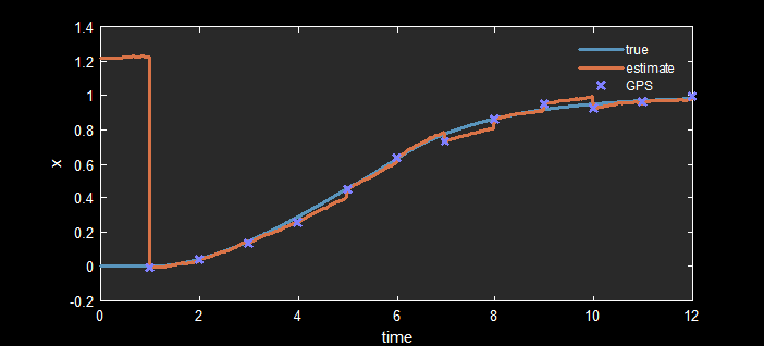
Notes:

• without the GPS measurements the double integration of accelerometer data will accumulate error over time
• the noise in the accelerometer is apparent in the wobbly estimate data between GPS updates
• this simulation iterates at 100Hz with GPS data every second