Octave/Matlab Control

Special thanks to Steve Brunton’s Control Bootcamp

These notes assume we have a linearized state-space representation of a system:

\[\begin{aligned} \\ \dot{x} &= Ax + Bu \\ y &= Cx + Du \\ \end{aligned}\]

And we want to design a controller \(K\):

\[u = -Ky\]

Feedback effectively changes the system dynamics to:

\[A - BK\]

Linear Math Commands

[v, lambda] = eig(A) # Get eigen vectors/eigen values of A
rank(A) # Get the rank of A
det(A)  # Get the determinant of A (note: det != 0 => A is full rank)

Feedback Control Basics

Controllability

To check if a system is controllable:

U = ctrb(A, B) # If U is full rank, system is controllable

Placing eigen values

If the system is controllable, we can place the eigen values of \((A - BK)\) wherever we like using:

K = place(Au, B, eig_spec);

Linear Quadratic Regulator

The LQR lets us determine \(K\) using a cost function. That is, what states should converge the fastest, and how conservative should we be with our controller.

\(Q\) and \(R\) are diagonal matricies.

Each diagonal value of \(Q\) weights the convergence of each state; the higher the value, the higher priority that state gets from the controller.

Each diagonal value of \(R\) weights the cost of using each control input; the higher the value, the more conservative the controller will be with that control input.

# Four states, single input
Q = [1 0 0 0; 0 1 0 0; 0 0 10 0; 0 0 0 100];
R = [0.01];
K = lqr(A, B, Q, R);

Sensing

Observability

The matrix \(C\) in \(y = Cx\) determines what states we can observe.

To determine if all states are observable, see if the observability matrix is full-rank:

obsv(A, C)

If it isn’t full rank, we may want to add/change sensors.

We may also want to check which states are the best to observe. To do this, we could try different \(C\) matrices, and then look at the determinant of the system observability gramian for a system.

sys = ss(A, B, C, D)
det(gram(sys, 'o')) # 'o' for observability
[vec, val] = eig(gram(sys, 'o'))

The determinant effectively calculates the volume of the \(\mathbb{R}^N\) spheriod represented by the grammian, the large the volume, the more observable our states. It is possible that this number can be deceptive if one eigen value is overrepresented; we should also check the eigen values to be sure.

Note: to calculate the gramian, \(A\) must be stable - in the inverted pendulum problem, this is acheived by modelling \(A\) for the case where the pendulum is low rather than upright.

Linear Quadratic Estimator (Kalman Filter)

The Kalman Filter takes a model and noise/disturbance estimations to compute an appropriate filter for observing system states.

The mechanism for this is simialar to the Linear Quadratic Regulator, except for a Linear Quadratic Estimator, our cost functions are defined in terms of a state disturbance matrix \(V_d\) and a sensor noise matrix \(V_n\).

Like \(Q\) and \(R\), both \(V_d\) and \(V_n\) are diagonal matrices, but with diagonal elements representing state disturbance and sensor noise respectively.

Vd = 0.1 * eye(4);
Vn = [1.0];
[Kf, P, E] = lqe(A, Vd, C, Vd, Vn);

Simulating a system

Given a system:

\[\begin{aligned} \\ \dot{x} &= Ax + Bu \\ y &= Cx + Du \\ \end{aligned}\]

We store the state space and simulate it with:

t = 0.0:0.01:10.0; # Define a time series [0.0, 10.0]s
sys = ss(A, B, C, D);
[y, t] = lsim(sys, u, t);
figure(); plot(t, y);

Adding noise and disturbance

To add noise and disturbance to our system, we treat them as additional inputs. That is, we add \(V_d\) and \(V_n\) to the \(B\) and \(D\) matrices.

BObs = [B, Vd, 0 * B];        # u | d | n
DObs = [0, 0, 0, 0, 0, Vn];   # u | d(1x4) | n

sysObs = ss(A, BObs, C, DObs); # Observable system

# Generate the gaussian disturbance and noise inputs
uDIST = randn(4, size(t, 2));
uNOISE = randn(size(t));

# Append disturbance and noise to u
uObs = [u; Vd*Vd*uDIST; uNOISE];

# Simulate
[y, t] = lsim(sysObs, uObs, t);
figure(); plot(t, y);

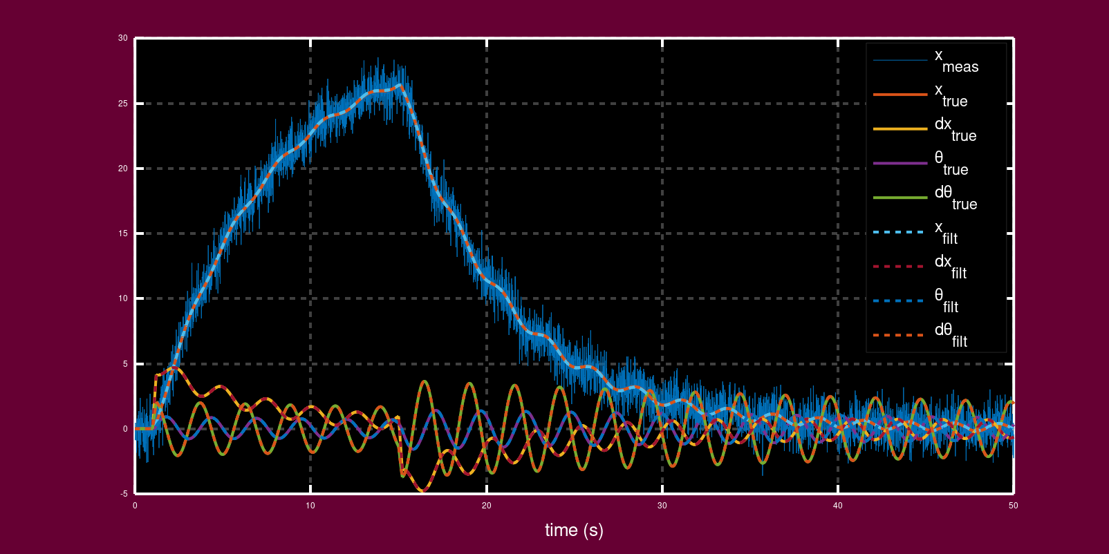
Simulating how well a Kalman filter tracks state

The following is adapted from Steve Brunton’s video; these are just some short hand notes to help me implement it myself when I need a reminder - I recommend watching the full video to understand how it comes together.

Define a system with full state output (i.e. we measure everything with perfect sensors):

CFull = eye(4);  # Perfect sensor!
# DFull: 4 states, 6 inputs - all zero!
DFull = zeros(4, sizeof(BObs, 2)); 
sysFull = ss(A, BObs, CFull, DFull);

Define a system which applies the Kalman filter \(K_f\) to estimate state:

BKf = [B, Kf];
CKf = eye(4);  # Represents KF outputs
sysKf = ss(A - Kf * C, BKf, eye(4), 0 * BKf);

Simulate the noisy system, then pass the output \(y\) through a the Kalman filter system:

[y, t] = lsim(sysObs, uObs', t);
[xFilt, t] = lsim(sysKf, [u; y']', t);

Simulate the true output:

[xTrue, t] = lsim(sysFull, uObs', t); 

Plot and compare the \(x_{true}\) with \(x_{filt}\):

plot(t, y, ...
    t, xtrue, 'LineWidth', 2.0, ...
    t, xFilt, '--', 'LineWidth', 2.0);

The filtered values should be overlaid on top of the true observations: