
Pendulum on cart derivation
In this guide, we derive the state space representation for a pendulum on a cart using Lagrange’s equations:
\[L = T - V\] \[\frac{d}{dt}\left(\frac{\partial L}{\partial \dot{q_i}}\right) - \frac{\partial L}{\partial q_i} = Q_i\]Free body diagram
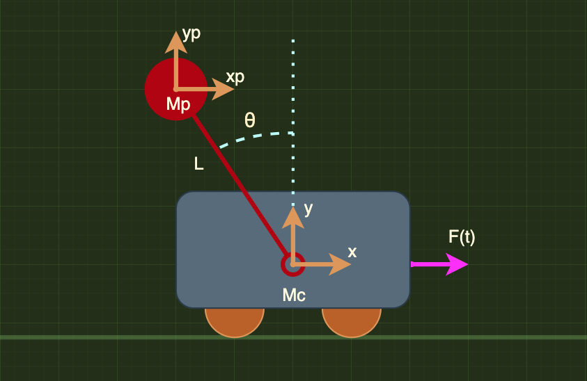
There are two sets of masses:
- \(M_c\); the cart mass
- \(\dot{y} = y = 0\); i.e. we don’t expect the cart to move in the y direction
- \(M_p\); the pendulum mass
- \(x_p = x + L \sin{\theta}\); the pendulum x-position
- \(\dot{x_p} = \dot{x} + L \cos{\theta}\); the pendulum x-velocity
- \(y_p = L \cos{\theta}\); the pendulum y-position
- \(\dot{y_p} = - L \sin{\theta}\); the pendulum y-velocity
System Kinetic Energy, T
\[\begin{aligned} T &= \frac{1}{2} M_c \dot{x}^2 + \frac{1}{2} M_p (\dot{x_p}^2 + \dot{y_p}^2) \\ &= \frac{1}{2}\dot{x}^2(M_c + M_p) - M_p L \dot{x}\dot{\theta}\cos{\theta} + \frac{1}{2} L^2 \dot{\theta}^2 M_p \end{aligned}\]System Potential Energy, V
\[\begin{aligned} V &= g M_p y_p \\ &= g M_p L \cos{\theta} \end{aligned}\]Lagrangian, L = T - V
\[L = \frac{1}{2}\dot{x}^2(M_c + M_p) - M_p L \dot{x}\dot{\theta}\cos{\theta} + \frac{1}{2} L^2 \dot{\theta}^2 M_p - g M_p L \cos{\theta}\]Forces
In the \(x\) coordinate:
\(F_x = F(t) - d_c \dot{x}\)
- Where: \(d_c \dot{x}\) is the cart dampening
In the \(\theta\) coordinate:
\(F_{\theta} = - d_p \dot{\theta}\)
- Where: \(d_c \dot{x}\) is the pendulum dampening
Equations of motion
We now want to solve:
\[\frac{d}{dt}\left(\frac{\partial L}{\partial \dot{q_i}}\right) - \frac{\partial L}{\partial q_i} = Q_i\]Where:
- \(q_i\) represents a coordinate in a system
- i.e. in our case, we have \((q_1, q_2) = (x, \theta)\)
- \(Q_i\) are the forces acting on the \(i^{th}\) coordinate
- i.e. in our case, we have \((Q_1, Q_2) = (F_x, F_{\theta})\)
Equations of motion w.r.t x
\[L = \frac{1}{2}\dot{x}^2(M_c + M_p) - M_p L \dot{x}\dot{\theta}\cos{\theta} + \frac{1}{2} L^2 \dot{\theta}^2 M_p - g M_p L \cos{\theta}\] \[\frac{d}{dt}\left(\frac{\partial L}{\partial \dot{x}}\right) - \frac{\partial L}{\partial x} = F_x\]So,
\[\begin{aligned} \frac{\partial L}{\partial \dot{x}} &= (M_c + M_p)\dot{x} - M_p L \dot{\theta} \cos{\theta} \\ \frac{d}{dt}\left(\frac{\partial L}{\partial \dot{x}}\right) &= (M_c + M_p)\ddot{x} - M_p L \ddot{\theta} \cos{\theta} + M_p L \dot{\theta}^2 \sin{\theta} \\ \frac{\partial L}{\partial x} &= 0 \end{aligned}\]Therefore:
\[(M_c + M_p)\ddot{x} - M_p L \ddot{\theta} \cos{\theta} + M_p L \dot{\theta}^2 \sin{\theta} = F(t) - d_c \dot{x}\]Equations of motion w.r.t \(\theta\)
\[L = \frac{1}{2}\dot{x}^2(M_c + M_p) - M_p L \dot{x}\dot{\theta}\cos{\theta} + \frac{1}{2} L^2 \dot{\theta}^2 M_p - g M_p L \cos{\theta}\] \[\frac{d}{dt}\left(\frac{\partial L}{\partial \dot{\theta}}\right) - \frac{\partial L}{\partial \theta} = F_{\theta}\]So,
\[\begin{aligned} \\ \frac{\partial L}{\partial \dot{\theta}} &= -M_p L \dot{x} \cos{\theta} + L^2 \dot{\theta} M_p \\ \frac{d}{dt}\left(\frac{\partial L}{\partial \dot{\theta}}\right) &= -M_p L (\ddot{x} \cos{\theta} - \dot{x}\dot{\theta}\sin{\theta}) + L^2 \ddot{\theta} M_p \\ \frac{\partial L}{\partial \theta} &= \dot{x} \dot{\theta} M_p L \sin{\theta} + g M_p L \sin{\theta} \\ \end{aligned}\]Therefore:
\[L \ddot{\theta} - \ddot{x}\cos{\theta} - g\sin{\theta} = -\dot{\theta}\frac{d_p}{M_p L}\]State space representation
Our equations of motion are:
\[(M_c + M_p)\ddot{x} - M_p L \ddot{\theta} \cos{\theta} + M_p L \dot{\theta}^2 \sin{\theta} = F(t) - d_c \dot{x}\] \[L \ddot{\theta} - \ddot{x}\cos{\theta} - g\sin{\theta} = -\dot{\theta}\frac{d_p}{M_p L}\]After a lot of rearranging:
\[\begin{aligned} \\ \ddot{x} &= \frac{F(t) - \dot{x} d_c - \dot{\theta}^2 M_p L \sin{\theta} - \dot{\theta}\frac{d_p}{L}\cos{\theta} + g M_p \cos{\theta}\sin{\theta}}{M_c + M_p - M_p\cos^2{\theta}} \\ \\ \ddot{\theta} &= \frac{1}{L}\frac{(F(t) - \dot{x} d_c - \dot{\theta}^2 M_p L \sin{\theta})\cos{\theta} - \dot{\theta} d_p \frac{M_c + M_p}{M_p L} + g (M_c + M_p) \sin{\theta}}{M_c + M_p - M_p\cos^2{\theta}} \\ \end{aligned}\]We can now represent this in an ode solver:
import scipy.integrate as integrate
import matplotlib.pyplot as plt
from matplotlib.gridspec import GridSpec
from matplotlib.animation import FuncAnimation
import numpy as np


class PendulumCart():
    def __init__(self, L=1.0, mP=1.0, mC=5.0, dP=0.0, dC=0.000, g=9.81):
        self.L = L
        self.mP = mP
        self.mC = mC
        self.dP = dP
        self.dC = dC
        self.g = g

    def _ode(self, X0, t,  inputT, inputF):
        x = X0[0]
        dx = X0[1]
        theta = X0[2]
        dtheta = X0[3]

        F = np.interp(t, inputT, inputF)

        s = np.sin(theta)
        c = np.cos(theta)

        num1 = F - (self.dC * dx) + \
            (self.mP * self.L * s * dtheta ** 2.0)
        num2 = c * self.g * s + \
            -(c * self.dP * dtheta) / (self.L)
        num3 = (self.mC + self.mP) * self.g * s + \
            -(self.mC + self.mP) * (self.dP * dtheta) / (self.mP * self.L)
        den = self.mC - (self.mP * s**2.0)

        ddx = (num1 + num2) / den
        ddtheta = (1/self.L) * (num1 * c + num3) / den

        dX = np.zeros(np.size(X0))
        dX[0] = dx
        dX[1] = ddx
        dX[2] = dtheta
        dX[3] = ddtheta

        return dX

    def simulate(self, x_init, t, inputT, inputF):
        return integrate.odeint(self._ode, x_init, t, (inputT, inputF))


class DrawCart:
    def __init__(self, ax, cart):
        with plt.style.context("dark_background"):
            self.body, = ax.plot([], [])
            self.arm, = ax.plot([], [])
            self.pen, = ax.plot([], [])
            self.ax = ax
            self.cart = cart
            ax.grid(True, linestyle=":", alpha=0.5)

    def draw(self, pos, theta):
        bh, bv = 0.5, 0.25
        bodyx = np.array([-1.0, -1.0, 1.0, 1.0, -1.0])*bh + pos
        bodyy = np.array([-1.0, 1.0, 1.0, -1.0, -1.0])*bv
        self.body.set_data(bodyx, bodyy)

        xp, yp = pos - np.sin(theta), np.cos(theta)
        self.arm.set_data([pos, xp], [0, yp])

        phi = np.linspace(-np.pi, np.pi, 32)
        d = self.cart.mP/self.cart.mC

        self.pen.set_data(xp + d*np.cos(phi), yp + d*np.sin(phi))

        self.ax.set_xlim(pos - 3, pos + 3)
        self.ax.set_ylim(-4, 4)
        return self.ax, self.body, self.arm, self.pen


cart = PendulumCart(L=1.0, mP=2.0, mC=10.0, dP=1.0, dC=5.0)

T0 = 0.0
TN = 10.0
t = np.linspace(T0, TN, num=5000)

x_init = [0.0, 0.0, np.pi*0.1, 0.0]

inputT = [T0, 5.0, 5.001, 5.5, 5.501, TN]
inputF = [0.0, 0.0, 200.0, 200.0, 0.0, 0.0]

x = cart.simulate(x_init, t, inputT, inputF)

with plt.style.context("dark_background"):
    color1 = plt.rcParams['axes.prop_cycle'].by_key()['color'][0]
    color2 = plt.rcParams['axes.prop_cycle'].by_key()['color'][1]
    color3 = plt.rcParams['axes.prop_cycle'].by_key()['color'][2]
    color4 = plt.rcParams['axes.prop_cycle'].by_key()['color'][3]
    color5 = plt.rcParams['axes.prop_cycle'].by_key()['color'][4]
    color6 = plt.rcParams['axes.prop_cycle'].by_key()['color'][5]

    fig = plt.figure(figsize=(10, 5))
    gs = GridSpec(3, 2, figure=fig)
    ax0 = fig.add_subplot(gs[:, 0])
    ax1 = fig.add_subplot(gs[0, 1])
    ax11 = ax1.twinx()
    ax2 = fig.add_subplot(gs[1, 1])
    ax21 = ax2.twinx()
    ax3 = fig.add_subplot(gs[2, 1])

points = np.full(5, None)

ax1.plot(t, x[:, 0], color=color1)

ax1.set_ylabel(r'x (m)', color=color1)
ax11.plot(t, x[:, 1], color=color2)

ax11.set_ylabel(r'$\dot{x}$ ($\frac{m}{s}$)', color=color2)

ax2.plot(t, x[:, 2], color=color3)
ax2.set_ylabel(r'$\theta$ (rad)', color=color3)
ax21.plot(t, x[:, 3], color=color4)
ax21.set_ylabel(r'$\dot{\theta}$ ($\frac{rad}{s}$)', color=color4)

ax3.plot(inputT, inputF, ':', color=color5)
ax3.set_ylabel(r'F (N)', color=color5)

dc = DrawCart(ax0, cart)

points[0], = ax1.plot([], [], 'o', color=color1)
points[1], = ax11.plot([], [], 'o', color=color2)
points[2], = ax2.plot([], [], 'o', color=color3)
points[3], = ax21.plot([], [], 'o', color=color4)
points[4], = ax3.plot([], [], 'o', color=color5)


def animate(i):
    time = (i % 100) * 0.1
    pos = np.interp(time, t, x[:, 0])
    dpos = np.interp(time, t, x[:, 1])
    theta = np.interp(time, t, x[:, 2])
    dtheta = np.interp(time, t, x[:, 3])
    force = np.interp(time, inputT, inputF)

    points[0].set_data(time, pos)
    points[1].set_data(time, dpos)
    points[2].set_data(time, theta)
    points[3].set_data(time, dtheta)
    points[4].set_data(time, force)

    ax, l1, l2, l3 = dc.draw(pos, theta)

    return ax, points[0], points[1], points[2], points[3], points[4],


ani = FuncAnimation(fig, animate, interval=100, save_count=100)
#ani.save('odePendulumCart.gif', writer='imagemagick')

plt.show()